11. Adaptive Mesh Refinement
11.1 Introduction
What is Adaptive Mesh Refinement and why does it make sense to use it to simulate tsunamis?
Adaptive mesh refinement (AMR) serves as a valuable numerical technique in simulations, dynamically adjusting computational mesh resolution based on evolving solution features. This approach provides several overarching advantages.
AMR optimizes computational efficiency by strategically allocating grid points. This involves concentrating resources in regions of interest while reducing resolution in less critical areas. Consequently, this adaptive strategy yields significant computational savings compared to simulations employing a uniform mesh.
In terms of accuracy, AMR proves advantageous by maintaining high resolution in areas experiencing rapid changes or featuring important phenomena. This adaptability results in more precise and reliable simulation outcomes compared to those achieved with a fixed mesh.
Moreover, AMR contributes to reduced memory requirements. By utilizing a finer mesh only where necessary, memory demands are minimized. This is particularly beneficial for large-scale simulations where memory constraints often serve as limiting factors.
11.2 Essential data infrastructures
To avoid misunderstandings and to provide a basic overview of AMReX data structures, let us introduce the concept of
the data types we use. We will begin by providing a list of classes, allowing you to refer back to them as needed.
Afterwards, we will use a simple diagram to help you understand the construction and relationships between the different
data types used. Additional information is always available in the
AMReX documentation.
Basics
Box
“Box in AMReX_Box.H is the data structure for representing a rectangular domain in indexing space. Box is a
dimension-dependent class. It has lower and upper corners (represented by IntVect)
and an index type (represented by IndexType).
A Box contains no floating-point data.”[1]
BoxArray
“BoxArray is a class in AMReX_BoxArray.H for storing a collection of Boxes on a single AMR level. One can make a
BoxArray out of a single Box and then chop it into multiple Boxes. In AMReX, BoxArray is a global data structure.
It holds all the Boxes in a collection, even though a single process in a parallel run only owns some of the Boxes via
domain decomposition.”[2]
DistributionMapping
“DistributionMapping is a class in AMReX_DistributionMapping.H that describes which process owns the data living on the
domains specified by the Boxes in a BoxArray. Like BoxArray, there is an element for each Box in DistributionMapping,
including the ones owned by other parallel processes. One can construct a DistributionMapping object given a BoxArray,
or by simply making a copy.”[3]
BaseFab
“BaseFab is a class template for multidimensional array-like data structure on a Box. The template parameter
is typically basic types such as Real, int or char. The dimensionality of the array is AMREX_SPACEDIM (here 2) plus
one. The additional dimension is for the number of components.”[4]
Array4
“Array4 is a class template for accessing BaseFab data in a more array like manner.”[4]
FabArray
“FabArray<FAB> is a class template in AMReX_FabArray.H for a collection of FABs on the same AMR level associated
with a BoxArray. The template parameter FAB is usually BaseFab<T>.”[5]
MultiFab
“In AMReX, there are some specialized classes derived from FabArray. The most commonly used FabArray kind class
is MultiFab in AMReX_MultiFab.H derived from FabArray <FArrayBox>
(FArrayBox).”[5]
Geometry
“The Geometry class in`` AMReX_Geometry.H`` describes problem domain and coordinate system for rectangular problem
domains.”[6]
Structure
Basic structure
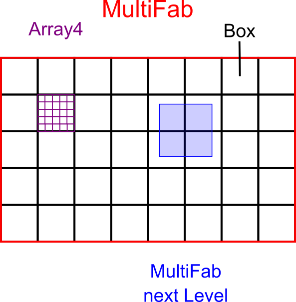
The MultiFab can be seen as a storage container for multiple boxes that are distributed over multiple processes managed by the DistributionMapping.
Each Box contains the array index required to iterate over the correct part of the underlying array.
Note that a Box does not include the index for ghost cells that are defined through the MultiFab.
The underlying array is called Array4 as it stores x, y, z dimension and an additional dimension for components.
The components are used to store multiple values in one Array4 respectively MultiFab.
E.g. In this project the components are used to store the height, momentum X, momentum Y, bathymetry and the error in one single MultiFab.
The next stage is realized by creating a new MultiFab, which stores boxes that do not extend over the entire domain.
These boxes are filled by the coarser underlying boxes.
Neighbouring Boxes in detail
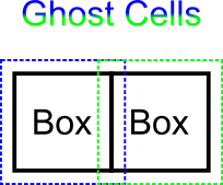
As mentioned before the boxes are distributed over the processes.
Therefore communication is needed to transfer data between boxes.
This is automatically done by AMReX by calling FillBoundary function.
The ghost cells are then typically filled with the data of valid cells, i.e. with the overlapping cells within the adjacent Box.
Subcycling & Level synchronization
Since we divide the cells to fine the level, the time step needs to be divided too to keep numerical accuracy. On the other hand, we need to synchronize the time step to transfer the data from fine to coarse and to fill new fine patches with data from the coarser level. To achieve this we use subscycling. The figure below shows the main concept for three AMR levels.
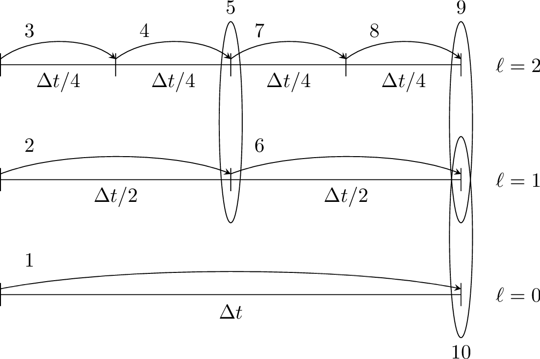
Therefore, we calculate the simulation in the following sequence of steps:
Advance \(\ell=0\) over \(\Delta t\).
Advance \(\ell=1\) over \(\Delta t/2\).
Advance \(\ell=2\) over \(\Delta t/4\).
Advance \(\ell=2\) over \(\Delta t/4\).
Synchronize levels \(\ell=1,2\).
Advance \(\ell=1\) over \(\Delta t/2\).
Advance \(\ell=2\) over \(\Delta t/4\).
Advance \(\ell=2\) over \(\Delta t/4\).
Synchronize levels \(\ell=1,2\).
Synchronize levels \(\ell=0,1\).
At the end one coarse step is finished, and we evolve to the next coarse time step.
To compensate for the mismatch in height, momentum X and momentum Y in levels \(\ell\) and \(\ell + 1\), we synchronise between these levels. “This is simply corrected by overwriting covered coarse cells to be the average of the overlying fine cells.”[7]
Flowchart
Here we want to give you a rough overview of the program. To do this, we have made a flowchart of the main functions that the program goes through. The next chapter explains the process in more detail and the steps the programme has to perform.

11.3 Code-Walkthrough
In this section, we want to explain the process of our program step by step, so that you can become familiar with the
code. We are going to start the course in our main.cpp file and follow along with the code.
AmrMesh and AmrCore
We use AmrMesh and AmrCore as the basic structure.
“For single-level simulations the user needs to build Geometry, DistributionMapping, and BoxArray objects
associated with the simulation. For simulations with multiple levels of refinement, the AmrMesh class can be thought
of as a container to store arrays of these objects (one for each level), and information about the current grid structure.”[8]
“AMReX_AmrCore.cpp/H contains the pure virtual class AmrCore, which is derived from the AmrMesh class.
AmrCore does not actually have any data members, just additional member functions, some of which override the base
class AmrMesh.”[8]
“There are no pure virtual functions in AmrMesh, but there are 5 pure virtual functions in the AmrCore class.
Any applications you create must implement these functions. The tutorial code Amr/Advection_AmrCore provides
sample implementation in the derived class AmrCoreAdv.”[8]
We will introduce them now because some of them are only called internally by AMReX functions, so we may not mention
them in the code walkthrough.
ErrorEst
To refine cells, this method uses TagBoxArray tags built on level grids. The refinement process begins by
calculating an error with the kernel state_error, and then tagging the cells accordingly.
Do not be overwhelmed by this block of code.
/// File:     'root/src/amr/AMRCoreWavePropagation2d.cpp'
/// Function: 'ErrorEst'

void tsunami_lab::amr::AMRCoreWavePropagation2d::ErrorEst( [ ... ] )
{
    [ ... ]
    for( MFIter mfi( state, false ); mfi.isValid(); ++mfi )
    {
        const Box& bx = mfi.validbox();

        Array4<const Real> height = state.const_array( mfi, HEIGHT );
        Array4<const Real> momentumX = state.const_array( mfi, MOMENTUM_X );
        Array4<const Real> momentumY = state.const_array( mfi, MOMENTUM_Y );
        Array4<const Real> bathymetry = state.const_array( mfi, BATHYMERTRY );
        Array4<Real> error = state.array( mfi, ERROR );
        const auto tagfab = tags.array( mfi );

        ParallelFor( bx,
                     [=] AMREX_GPU_DEVICE( int i, int j, int k ) noexcept
        {
            state_error( i, j, k, tagfab, height, momentumX, momentumY, bathymetry, error, gridError, tagval );
        } );
    }
}
Here we will explain the logic behind the MFIter and ParallelFor loop. We will skip this for
now because we do not want to throw you in at the deep end. It is only important at the moment that we call
state_error, which is our kernel function.
/// File:     'root/include/amr/Kernels.h'
/// Function: 'state_error

void state_error( [ ... ] )
{
    amrex::Real divHeight = 1 / height( i, j, k );
    amrex::Real velocityX = momentumX( i, j, k ) * divHeight;
    amrex::Real velocityY = momentumY( i, j, k ) * divHeight;
    amrex::Real waveHeight = height( i, j, k ) + bathymetry( i, j, k );
    error( i, j, k ) = ( velocityX * velocityX + velocityY * velocityY ) * waveHeight * waveHeight;
    // the gridErr is squared therefore we can use the error squared too
    tag( i, j, k ) = ( error( i, j, k ) > gridErr ) * tagval;
}
Our criteria for determining whether to tag the cell is in the first highlighted line. The calculation involves squaring the velocity in both the x and y directions and multiplying the result by the squared water height. The reason for using these criteria is simple. We debugged different characteristics of our cells and experimented with various combinations. We ended up with the best and most reliable criteria, which you can see here. Overall, it is logical that velocity and water height are descriptive properties.
In the second highlighted line, we either set or do not set the tag. The gridErr is defined in inputs.amrex
(tsunami.griderr) and varies depending on the level.
MakeNewLevelFromScratch
Make a new level from scratch using provided BoxArray and DistributionMapping. Only used during initialization.
Upon creating the simulation, the first level is initialized.
/// File:     'root/src/amr/AMRCoreWavePropagation2d.cpp'
/// Function: 'MakeNewLevelFromScratch'

void tsunami_lab::amr::AMRCoreWavePropagation2d::MakeNewLevelFromScratch( [ ... ] )
{

    // init the multifab
    gridNew[level].define( ba, dm, nComponents, nGhostRow );
    gridOld[level].define( ba, dm, nComponents, nGhostRow );

    // set the time
    tNew[level] = time;
    tOld[level] = time - dt[level];

    InitData( level );
}
MakeNewLevelFromCoarse
Make a new level using provided BoxArray and DistributionMapping and fill with interpolated coarse level data.
This phrase is used whenever a new level needs to be created. For example, to create a refinement of level 3, we must
create a level from level 2, which is considered coarse in this case.
/// File:     'root/src/amr/AMRCoreWavePropagation2d.cpp'
/// Function: 'MakeNewLevelFromCoarse'

void tsunami_lab::amr::AMRCoreWavePropagation2d::MakeNewLevelFromCoarse( [ ... ] )
{
    // init the multifab
    gridNew[level].define( ba, dm, nComponents, nGhostRow );
    gridOld[level].define( ba, dm, nComponents, nGhostRow );

    // set the time
    tNew[level] = time;
    tOld[level] = time - dt[level];

    FillFinePatch( level, time, gridNew[level] );
}
FillFinePatch is a helper function. The entire MultiFab is filled by interpolating from the coarser level when
a new level of refinement appears.
/// File:     'root/src/amr/AMRCoreWavePropagation2d.cpp'
/// Function: 'FillFinePatch'

void tsunami_lab::amr::AMRCoreWavePropagation2d::FillFinePatch( [ ... ] )
{
    [ ... ]
    // decomp is the starting component of the destination. Therefore scomp = dcomp
    InterpFromCoarseLevel( mf, time, *cmf[0], 0, 0, 4, geom[level - 1], geom[level],
                           cphysbc, 0, fphysbc, 0, refRatio( level - 1 ),
                           interpolator, physicalBoundary, 0 );

    // do a piecewise constant interpolation to fill cell near the shore i.e. |bathymetry| < bathymetryMinValue
    MultiFab tmf( mf.boxArray(), mf.DistributionMap(), 4, mf.nGrow() );
    InterpFromCoarseLevel( tmf, time, *cmf[0], 0, 0, 4, geom[level - 1], geom[level],
                           cphysbc, 0, fphysbc, 0, refRatio( level - 1 ),
                           &pc_interp, physicalBoundary, 0 );

    FixFinePatch( mf, tmf );
}
The last line FixFinePatch fixes the MultiFab interpolation from the coarser level. This is relevant when
the fine level is created or updated. It replaces the values of mf with const_mf for the cell near the shore where
|bathymetry| < bathymetryMinValue and set the height on the coast to zero. To prevent the issue of dry-wet, this is
necessary.
RemakeLevel
Remake an existing level using provided BoxArray and DistributionMapping and fill with existing fine and coarse
data.
/// File:     'root/src/amr/AMRCoreWavePropagation2d.cpp'
/// Function: 'RemakeLevel'

void tsunami_lab::amr::AMRCoreWavePropagation2d::RemakeLevel( [ ... ] )
{
    MultiFab new_state( ba, dm, nComponents, nGhostRow );
    MultiFab old_state( ba, dm, nComponents, nGhostRow );

    FillPatch( level, time, new_state );

    std::swap( new_state, gridNew[level] );
    std::swap( old_state, gridOld[level] );

    tNew[level] = time;
    tOld[level] = time - dt[level];
}
ClearLevel
This function deletes level data to clean up.
/// File:     'root/src/amr/AMRCoreWavePropagation2d.cpp'
/// Function: 'ClearLevel'

void tsunami_lab::amr::AMRCoreWavePropagation2d::ClearLevel( int level )
{
    gridNew[level].clear();
    gridOld[level].clear();
}
Initialize & Finalize
“To use AMReX, we need to call Initialize to initialize the execution environment for AMReX, and Finalize needs
to be paired with Initialize to free the resources used by AMReX. Because many AMReX classes and functions don’t work
properly after amrex::Finalize is called, it’s best to put the code between amrex::Initialize and amrex::Finalize in its
scope to make sure that resources are freed properly”[9].
/// File: 'root/src/main.cpp'

int main( int /*i_argc*/, char* i_argv[] )
{
    [ ... ]
    amrex::Initialize( argc, argv )
    { ... }
    amrex::Finalize();
    return EXIT_SUCCESS;
}
ParmParse
Before starting a simulation, the user must define its configuration. To simplify this process, you only need to adjust
the parameters in the root/resources/inputs.amrex file. “We use the AMReX class AMReX_ParmParse.H, which
provides a database for storing and retrieving command line and input file arguments”[10]. This technique is used
throughout the project to get the correct parameters when they are needed. Here is an example of how to get the
displacement and bathymetry file paths:
/// File: 'root/src/main.cpp'

[ ... ]
amrex::ParmParse ppTsunami( "tsunami" );
std::string bathymetryFile;
std::string displacementFile;
ppTsunami.query( "bathymetry_file", bathymetryFile );
ppTsunami.query( "displacement_file", displacementFile );
[ ... ]
The setup and preparation process of the simulation starts by initializing our AMRCoreWavePropagation2d.
/// File: 'root/src/main.cpp'

[ ... ]
tsunami_lab::amr::AMRCoreWavePropagation2d* waveProp = new tsunami_lab::amr::AMRCoreWavePropagation2d( setup );
[ ... ]
InitFromScratch
The constructor invokes the ReadParameters function to obtain the input file parameters and resizes them to the
maximum level, nLevelMax. Therefore, if we declare parameters in our inputs.amerx file for levels one to five,
but only have a maximum of three levels, we will only require the first three entries in the vectors. We then set the
refinement ratio for each level and fill our boundaries. To initialize our data, we pass the
start time, which is still zero, to InitFromScratch.
/// File:     'root/src/amr/AMRCoreWavePropagation2d.cpp'
/// Function: 'AMRCoreWavePropagation2d'

ReadParameters();
//resize to the levels
[ ... ]
// set the refinement ratio for each level for subcycling
for( int lev = 1; lev <= max_level; ++lev )
{
    nSubSteps[lev] = MaxRefRatio( lev - 1 );
}

// set the interpolation method
for( int dim = 0; dim < AMREX_SPACEDIM; ++dim )
{
    for( int n = 0; n < nComponents; ++n )
    {
        physicalBoundary[n].setLo( dim, BCType::foextrap );
        physicalBoundary[n].setHi( dim, BCType::foextrap );
    }
}

// init the domain
InitFromScratch( 0.0 );
This initializes BoxArray, DistributionMapping and data from scratch. Calling this function requires the derived class
implement its own MakeNewLevelFromScratch (root/src/amr/AMRCoreWavePropagation2d.cpp) to allocate and initialize data.
This method makes a new level from scratch using provided BoxArray and DistributionMapping and then calls
InitData to initialize our data structures.
InitData
The data from the setup is read into the grid by InitData. To accomplish this, we will now provide a detailed
explanation of how to loop over the grid and access its cells. Working with AMReX will require this as a prerequisite.
 1/// File:     'root/src/amr/AMRCoreWavePropagation2d.cpp'
 2/// Function: 'InitData'
 3
 4[ ... ]
 5for( MFIter mfi( gridNew[level], false ); mfi.isValid(); ++mfi )
 6{
 7    Box bx = mfi.validbox();
 8
 9    Array4<Real> height = gridNew[level].array( mfi, HEIGHT );
10    Array4<Real> momentumX = gridNew[level].array( mfi, MOMENTUM_X );
11    Array4<Real> momentumY = gridNew[level].array( mfi, MOMENTUM_Y );
12    Array4<Real> bathymetry = gridNew[level].array( mfi, BATHYMERTRY );
13
14    ParallelFor( bx,
15                [=] AMREX_GPU_DEVICE( int i, int j, int k )
16    {
17        Real x = i * dx;
18        Real y = j * dy;
19        height( i, j, k ) = setup->getHeight( x, y );
20        momentumX( i, j, k ) = setup->getMomentumX( x, y );
21        momentumY( i, j, k ) = setup->getMomentumY( x, y );
22        bathymetry( i, j, k ) = setup->getBathymetry( x, y );
23    } );
24}
25[ ... ]
“Above we see how you can operate on the MultiFab data with your own functions. AMReX provides an iterator, MFIter
for looping over the FArrayBoxes in MultiFabs. MFIter only loops over grids owned by this process.”[11]
Tiling is not being used in this MFiter loop because it was set to false in line five. Tiling improves data
locality when loading data that is not directly consecutive in memory. One way to achieve this is by transforming loops into tiling loops that iterate over tiles and element loops
that iterate over the data elements within a tile. We use tiling only where it makes sense. For example, it improves our
ySweep but not our xSweep, which will be introduced later.
Passing
truewhen definingMFIterto indicate tiling.Calling
tileboxinstead ofvalidboxto obtain the tiled work region for the loop iteration.
To simplify data management, we create an Array4 for each component that holds its specific values.
Currently, we are only iterating over the Boxes of our MultiFab. In order to iterate over the cells,
we will use ParallelFor. “ParallelFor takes two arguments. The first argument is a Box specifying the
iteration index space, and the second argument is a C++ lambda function that works on cell (i, j, k).”[12]
Evolve
We have completed the setup of our simulation and returned to our main.cpp. Let’s jump into
AMRCoreWavePropagation2d.cpp where the real simulation is done. Our starting point is
/// File: 'root/src/main.cpp'

waveProp->Evolve();
WritePlotFile
The Evolve method progresses through time step by step using a loop. The program determines independently whether to
generate a plot file at the start. We call WritePlotFile to write a simulation step.
/// File:     'root/src/amr/AMRCoreWavePropagation2d.cpp'
/// Function: 'Evolve'

[ ... ]
if( currentTime >= writes * writeFrequency )
{
    writes++;
    WritePlotFile();
}
[ ... ]
The tsunami-specific values ‘Height’, ‘MomentumX’, ‘MomentumY’, ‘Bathymetry’, and ‘Error’ are defined in WritePlotFile
and are intended to be saved in the plot. We call the provided function WriteMultiLevelPlotfile to create the actual
plot. “AMReX has its own native plotfile format. Many visualization tools are available for AMReX plotfiles”[13].
We used ParaView to visualize the plot files with confidence. If you want to get more information about this we
recommend the chapter Visualization.
timeStepWithSubcycling
timeStepWithSubcycling advances a level by dt, includes a recursive call for finer levels. First of all we check
if we want to regrid. To regrid, three conditions must be met. The current level must be lower than the maximum
refinement level max_level. Then we have to be sure that we don’t regrid fine levels again if it was taken care of
during a coarse regird. Additionally, we need to check if it is time to regrid based on the regridFrequency variable,
which defines the number of time steps between each regrid.
/// File:     'root/src/amr/AMRCoreWavePropagation2d.cpp'
/// Function: 'timeStepWithSubcycling'

[ ... ]
if( level < max_level
    && step[level] > lastRegridStep[level]
    && step[level] % regridFrequency == 0 )
{
    // regrid could add newly refine levels (if finest_level < max_level)
    // so we save the previous finest level index
    int oldFinest = finest_level;
    regrid( level, time );

    // mark that we have regridded this level already
    for( int k = level; k <= finest_level; ++k )
    {
        lastRegridStep[k] = step[k];
    }

    // if there are newly created levels, set the time step
    for( int k = oldFinest + 1; k <= finest_level; ++k )
    {
        dt[k] = dt[k - 1] / MaxRefRatio( k - 1 );
    }
}
[ ... ]
If regridding is necessary, we use the internal method regrid. MakeNewGrids will be invoked by this method,
which will use ErrorEst to tag the cells for regridding. Afterwards, RemakeLevel is called to remake an existing
level using the provided BoxArray and DistributionMapping, and fill it with existing fine and coarse data.
Then, MakeNewLevelFromCoarse is called to create a new level using the provided BoxArray and
DistributionMapping, and fill it with interpolated coarse level data. At this point, a new refinement level is
created. ClearLevel is then used to delete level data at the end.
/// File:     'root/submodules/amrex/Src/AmrCore/AMReX_AmrCore.cpp'
/// Function: 'regrid'

void AmrCore::regrid (int lbase, Real time, bool)
{
    if (lbase >= max_level) { return; }

    int new_finest;
    Vector<BoxArray> new_grids(finest_level+2);
    MakeNewGrids(lbase, time, new_finest, new_grids);

    BL_ASSERT(new_finest <= finest_level+1);

    bool coarse_ba_changed = false;
    for (int lev = lbase+1; lev <= new_finest; ++lev)
    {
        if (lev <= finest_level) // an old level
        {
            bool ba_changed = (new_grids[lev] != grids[lev]);
            if (ba_changed || coarse_ba_changed) {
                BoxArray level_grids = grids[lev];
                DistributionMapping level_dmap = dmap[lev];
                if (ba_changed) {
                    level_grids = new_grids[lev];
                    level_dmap = MakeDistributionMap(lev, level_grids);
                }
                const auto old_num_setdm = num_setdm;
                RemakeLevel(lev, time, level_grids, level_dmap);
                SetBoxArray(lev, level_grids);
                if (old_num_setdm == num_setdm) {
                    SetDistributionMap(lev, level_dmap);
                }
            }
            coarse_ba_changed = ba_changed;;
        }
        else  // a new level
        {
            DistributionMapping new_dmap = MakeDistributionMap(lev, new_grids[lev]);
            const auto old_num_setdm = num_setdm;
            MakeNewLevelFromCoarse(lev, time, new_grids[lev], new_dmap);
            SetBoxArray(lev, new_grids[lev]);
            if (old_num_setdm == num_setdm) {
                SetDistributionMap(lev, new_dmap);
            }
        }
    }

    for (int lev = new_finest+1; lev <= finest_level; ++lev) {
        ClearLevel(lev);
        ClearBoxArray(lev);
        ClearDistributionMap(lev);
    }

    finest_level = new_finest;
}
Since we already introduced most of these functions at the beginning of this chapter, we will
not provide a detailed explanation of them here. Furthermore, AMReX aims to implement these functions to ensure
compatibility with the framework. The above code provides an example of how the framework works using these methods.
After regridding, we advance one level for one time step by calling AdvanceGridAtLevel.
/// File:     'root/src/amr/AMRCoreWavePropagation2d.cpp'
/// Function: 'timeStepWithSubcycling'

[ ... ]
AdvanceGridAtLevel( level, time, dt[level], iteration, nSubSteps[level] );
[ ... ]
Before we go into this method, let us look at the last part of timeStepWithSubcycling. As the name suggests, we also
aim to progress through time on a smaller scale. To achieve this, we use the recursive procedure.
/// File:     'root/src/amr/AMRCoreWavePropagation2d.cpp'
/// Function: 'timeStepWithSubcycling'

[ ... ]
if( level < finest_level )
{
    // recursive call for next-finer level
    for( int i = 1; i <= nSubSteps[level + 1]; ++i )
    {
        timeStepWithSubcycling( level + 1, time + ( i - 1 ) * dt[level + 1], i );
    }

    // update level based on coarse-fine flux mismatch
    AverageDownTo( level ); // average level+1 down to level
}
As we can see, we are calling the subroutines and then using AverageDownTo to average down across multiple levels.
We defined this method ourselves to limit the arguments of the average_down method provided by AMReX.
/// File:     'root/src/amr/AMRCoreWavePropagation2d.cpp'
/// Function: 'AverageDownTo'

void tsunami_lab::amr::AMRCoreWavePropagation2d::AverageDownTo( int coarseLevel )
{
    // Average down the first 3 Components: Height, MomentumX, MomentumY
    average_down( gridNew[coarseLevel + 1], gridNew[coarseLevel],
                  geom[coarseLevel + 1], geom[coarseLevel],
                  0, 3, refRatio( coarseLevel ) );
}
AdvanceGridAtLevel
Let’s revisit AdvanceGridAtLevel and examine it more closely. This is the method to advance the grid by one level
for one time step. Before performing the x and y sweep, it is necessary to call FillPatch.
/// File:     'root/src/amr/AMRCoreWavePropagation2d.cpp'
/// Function: 'AdvanceGridAtLevel'

[ ... ]
// swapping the grid to keep the current time step in gridOld
// and advance with the MultiFab in gridNew
std::swap( gridOld[level], gridNew[level] );

MultiFab& state = gridNew[level];

// size in x & y direction
const Real dx = geom[level].CellSize( 0 );
const Real dy = geom[level].CellSize( 1 );

// scaling in each dimension
Real dtdx = dtLevel / dx;
Real dtdy = dtLevel / dy;

// State with ghost cells
MultiFab stateTemp( grids[level], dmap[level], 4, nGhostRow );
FillPatch( level, time, stateTemp );
state.ParallelCopy( stateTemp, 0, 0, 4, nGhostRow, nGhostRow );
[ ... ]
In AdvanceGridAtLevel, we create a temporary MultiFab called stateTemp, which is essentially our grid but
with ghost cells filled in. The valid and ghost cells are filled in from actual valid data at that level, space-time
interpolated data from the next-coarser level, neighboring grids at the same level, or domain boundary conditions.
FillPatch
This method is needed to fill a patch with data. The code includes two functions: FillPatchSingleLevel and
FillPatchTwoLevels. To enable this, we must first use our utility function, GetData. This method copies data from
gridOld and/or gridNew into another MultiFab for further use.
“
FillPatchSingleLevelfills aMultiFaband its ghost region at a single level of refinement. The routine is flexible enough to interpolate in time between twoMultiFabsassociated with different times.”[14]“
FillPatchTwoLevelsfills aMultiFaband its ghost region at a single level of refinement, assuming there is an underlying coarse level. This routine is flexible enough to interpolate the coarser level in time first usingFillPatchSingleLevel.”[14]
“Note that FillPatchSingleLevel and FillPatchTwoLevels call the single-level routines MultiFab::FillBoundary
and FillDomainBoundary to fill interior, periodic, and physical boundary ghost cells.”[14]
/// File:     'root/src/amr/AMRCoreWavePropagation2d.cpp'
/// Function: 'FillPatch'

[ ... ]
if( level == 0 )
{
    Vector<MultiFab*> smf;
    Vector<Real> stime;
    GetData( 0, time, smf, stime );

    CpuBndryFuncFab bndry_func( nullptr );  // Without EXT_DIR, we can pass a nullptr.
    PhysBCFunct<CpuBndryFuncFab> physbc( geom[level], physicalBoundary, bndry_func );
    // decomp is the starting component of the destination. Therefore scomp = dcomp
    FillPatchSingleLevel( mf, time, smf, stime, 0, 0, 4,
                          geom[level], physbc, 0 );
}
else
{
    Vector<MultiFab*> cmf, fmf;
    Vector<Real> ctime, ftime;
    GetData( level - 1, time, cmf, ctime );
    GetData( level, time, fmf, ftime );

    CpuBndryFuncFab bndry_func( nullptr );  // Without EXT_DIR, we can pass a nullptr.
    PhysBCFunct<CpuBndryFuncFab> cphysbc( geom[level - 1], physicalBoundary, bndry_func );
    PhysBCFunct<CpuBndryFuncFab> fphysbc( geom[level], physicalBoundary, bndry_func );

    // decomp is the starting component of the destination. Therefore scomp = dcomp
    FillPatchTwoLevels( mf, time, cmf, ctime, fmf, ftime,
                        0, 0, 4, geom[level - 1], geom[level],
                        cphysbc, 0, fphysbc, 0, refRatio( level - 1 ),
                        interpolator, physicalBoundary, 0 );

    // do a piecewise constant interpolation to fill cell near the shore i.e. |bathymetry| < bathymetryMinValue
    MultiFab tmf( mf.boxArray(), mf.DistributionMap(), 4, mf.nGrow() );
    FillPatchTwoLevels( tmf, time, cmf, ctime, fmf, ftime,
                        0, 0, 4, geom[level - 1], geom[level],
                        cphysbc, 0, fphysbc, 0, refRatio( level - 1 ),
                        &pc_interp, physicalBoundary, 0 );

    FixFinePatch( mf, tmf );
The second instance of FillPatchTwoLevels is required to fill cells near the coast and prevent the dry-wet problem.
This is necessary because our simulation is not capable of handling this issue. The last line FixFinePatch fixes the
MultiFab interpolation from the coarser level. This is relevant when the fine level is created or updated. It
replaces the values of mf with const_mf for the cell near the shore where |bathymetry| < bathymetryMinValue
and set the height on the coast to zero. To prevent the issue of dry-wet, this is also necessary.
A FillPatch uses an Interpolator. This is largely hidden from application codes. AMReX_Interpolater.cpp/H
contains the virtual base class Interpolater, which provides an interface for coarse-to-fine spatial interpolation
operators. The fillpatch routines described above require an Interpolater for FillPatchTwoLevels. In addition
to the special case, we are using the amrex::lincc_interp interpolator.
CellConservativeLinear lincc_interp
“Dimension-by-dimension linear interpolation with MC limiter for cell-centered data. For multi-component data, the strictest limiter is used for all components. For example, if one component after its own limiting has a slope of zero, all other components will have zero slopes as well eventually. The interpolation is conservative in finite-volume sense for both Cartesian and curvilinear coordinates.”[15]
Back in AdvanceGridAtLevel we finally do the x and y sweep of the cells.
/// File:     'root/src/amr/AMRCoreWavePropagation2d.cpp'
/// Function: 'AdvanceGridAtLevel'

[ ... ]
#ifdef AMREX_USE_OMP
#pragma omp parallel
#endif
    for( MFIter mfi( state, false ); mfi.isValid(); ++mfi )
    {
        // ===== UPDATE X SWEEP =====
        const Box& bx = mfi.validbox();

        // define the grid components
        Array4<Real const> height = state.const_array( mfi, HEIGHT );
        Array4<Real const> momentumX = state.const_array( mfi, MOMENTUM_X );
        Array4<Real const> bathymetry = state.const_array( mfi, BATHYMERTRY );
        Array4<Real      > gridOut = stateTemp.array( mfi );

        // compute the x-sweep
        launch( grow( bx, 1 ),
                [=] AMREX_GPU_DEVICE( const Box & tbx )
        {
            xSweep( tbx, dtdx, height, momentumX, bathymetry, gridOut );
        } );
    }

    state.ParallelCopy( stateTemp, 0, 0, 4, 0, 0 );
    state.FillBoundary();

#ifdef AMREX_USE_OMP
#pragma omp parallel
#endif
    for( MFIter mfi( state, true ); mfi.isValid(); ++mfi )
    {
        // ===== UPDATE Y SWEEP =====
        const Box& bx = mfi.tilebox();

        // swap the grid components
        Array4<Real const> height = stateTemp.const_array( mfi, HEIGHT );
        Array4<Real const> momentumY = stateTemp.const_array( mfi, MOMENTUM_Y );
        Array4<Real const> bathymetry = stateTemp.const_array( mfi, BATHYMERTRY );
        Array4<Real      > gridOut = state.array( mfi );

        // compute the y-sweep
        launch( grow( bx, 1 ),
                [=] AMREX_GPU_DEVICE( const Box & tbx )
        {
            ySweep( tbx, dtdy, height, momentumY, bathymetry, gridOut );
        } );
    }
The xSweep and ySweep are kernel methods declared in root/include/amr/Kernels.h. Both are very similar. We first
calculate the reflection and then compute the net-updates using our F-Wave solver to update the grid cells. Below is
the procedure for xSweep, which is analogous to ySweep.
/// File:     'root/include/amr/Kernels.h'
/// Function: 'xSweep'

void xSweep( [ ... ] )
{
    [ ... ]
    for( int j = lo.y; j < hi.y; ++j )
    {
        AMREX_PRAGMA_SIMD
            for( int i = lo.x; i < hi.x; ++i )
            {
                // noting to compute both shore cells
                if( height( i, j, 0 ) <= amrex::Real( 0.0 ) && height( i + 1, j, 0 ) <= amrex::Real( 0.0 ) )
                {
                    continue;
                }

                // calculate the reflection
                bool leftReflection = ( height( i + 1, j, 0 ) <= amrex::Real( 0.0 ) );
                amrex::Real heightRight = leftReflection ? height( i, j, 0 ) : height( i + 1, j, 0 );
                amrex::Real momentumRight = leftReflection ? -momentumX( i, j, 0 ) : momentumX( i + 1, j, 0 );
                amrex::Real bathymetryRight = leftReflection ? bathymetry( i, j, 0 ) : bathymetry( i + 1, j, 0 );

                bool rightReflection = ( height( i, j, 0 ) <= amrex::Real( 0.0 ) );
                amrex::Real heightLeft = rightReflection ? height( i + 1, j, 0 ) : height( i, j, 0 );
                amrex::Real momentumLeft = rightReflection ? -momentumX( i + 1, j, 0 ) : momentumX( i, j, 0 );
                amrex::Real bathymetryLeft = rightReflection ? bathymetry( i + 1, j, 0 ) : bathymetry( i, j, 0 );

                // compute net-updates
                tsunami_lab::t_real netUpdates[2][2];
                tsunami_lab::solvers::FWave::netUpdates( [ ... ] );

                gridOut( i, j, 0, Component::HEIGHT ) -= scaling * netUpdates[0][0] * !rightReflection;
                gridOut( i, j, 0, Component::MOMENTUM_X ) -= scaling * netUpdates[0][1] * !rightReflection;

                gridOut( i + 1, j, 0, Component::HEIGHT ) -= scaling * netUpdates[1][0] * !leftReflection;
                gridOut( i + 1, j, 0, Component::MOMENTUM_X ) -= scaling * netUpdates[1][1] * !leftReflection;
            }
    }
}
After completing the sweeps and finishing AverageDownTo, we have performed a cycle successfully. We now return to the
Evolve method to check if the current time is less than the time to simulate. If it is, we execute the next
timeStepWithSubcycling. If not, the simulation is complete.
We hope this code walkthrough was helpful in understanding the behavior and functionality of our adaptive mesh
refinement tsunami simulation. We covered all the methods we defined in AMRCoreWavePropagation2d. Of course, we use
functions of the AMReX framework. These are internal and could be used by us without modification. If you want to
learn more about AMReX and the functions it provides, we recommend you read the
source documentation and the
tutorial documentation.
But enough theory. Adaptive mesh refinement has two main goals that go hand in hand. We want to increase the accuracy of our simulation while maintaining good runtime performance. In the next two chapters we will test our program and take a closer look at the results and whether we have achieved the expected behavior.
11.4 Performance
Load Balancing
“Single-level load balancing algorithms are sequentially applied to each AMR level independently, and the resulting distributions are mapped onto the ranks taking into account the weights already assigned to them (assign heaviest set of grids to the least loaded rank). Note that the load of each process is measured by how much memory has already been allocated, not how much memory will be allocated.”[16]
AMReX provides three load balancing algorithms: Knapsack, SFC and Round-robin.
We kept the default algorithm SFC which “enumerate grids with a space-filling Z-morton curve, then partition the resulting ordering across ranks in a way that balances the load.”[16]
Benchmarks
This benchmark uses the Tohoku tsunami setup with 1000 m cells, writing every 60 seconds of simulation time.
Original is our last release that does not include AMReX, see
Submission 9. Parallelization.
This inputs.amrex configuration file was used for the AMR simulation with AMReX.
I/0 Enabled |
2 min 31 sec |
2 min 21 sec |
9 min 20 sec |
23 min 29 sec |
46 min 20 sec |
I/0 Disabled |
1 min 34 sec |
1 min 48 sec |
8 min 43 sec |
22 min 31 sec |
45 min 11 sec |
The levels are designated as follows: 1 level is the coarse level only, 2 levels has the coarse level and one additional fine level, 3 levels has the coarse level and two additional fine levels and so on. From one fine level to another, the cells are divided in half, i.e. one 1000 m cell becomes four 500 m cells. The levels therefore have the following sizes: Level 1 with 1000 m, Level 2 with 500 m, Level 3 with 250 m and Level 4 with 125 m.
The comparison of Original and 1 Level shows that the AMR implementation requires more computation for the
simulation itself. However, using the AMReX output format is faster than using the netCdf writer.
We also used the Original program to run on 250 m cells with I/O, which took 1 h 47 min 13 sec compared to
3 Levels which took only 23 min 29 sec. Using AMR to only partially refine the mesh we get a significant
performance increase with a speedup of 4.76.
11.5 Visualization
Accuracy
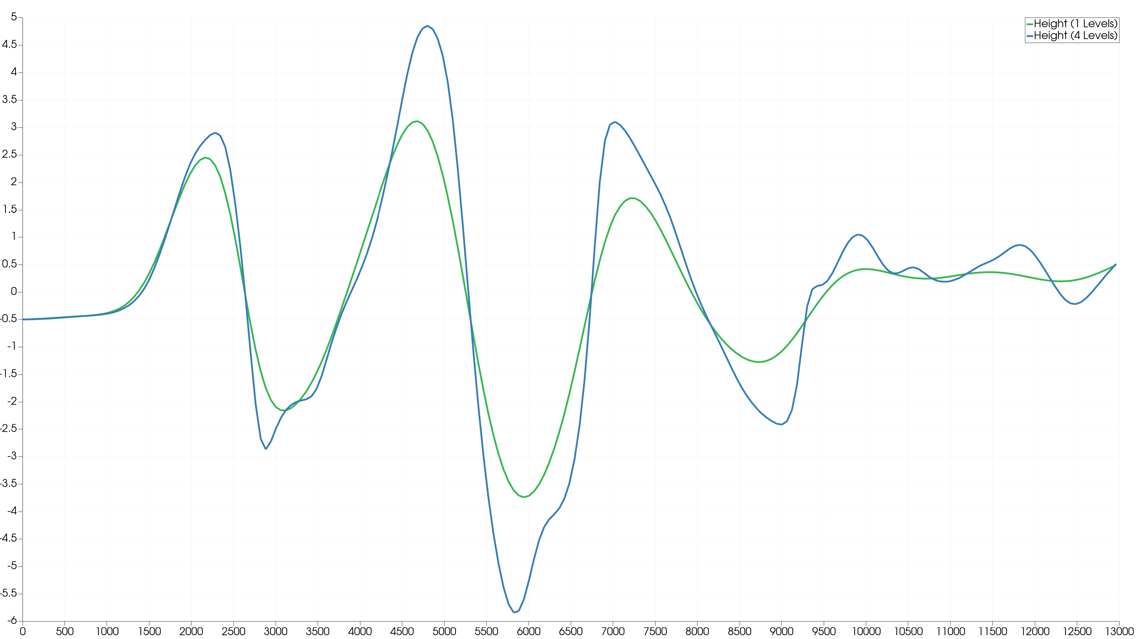
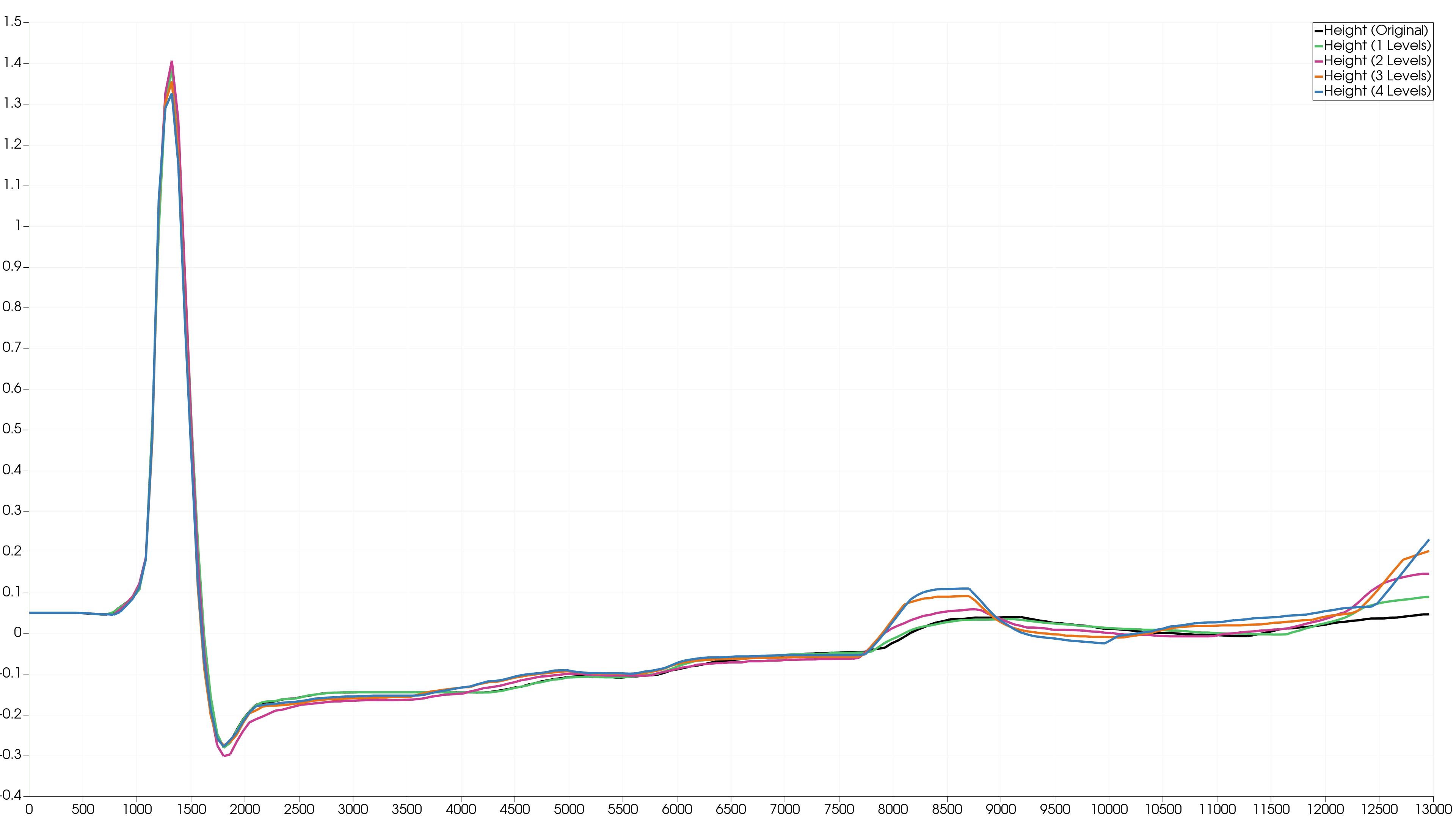
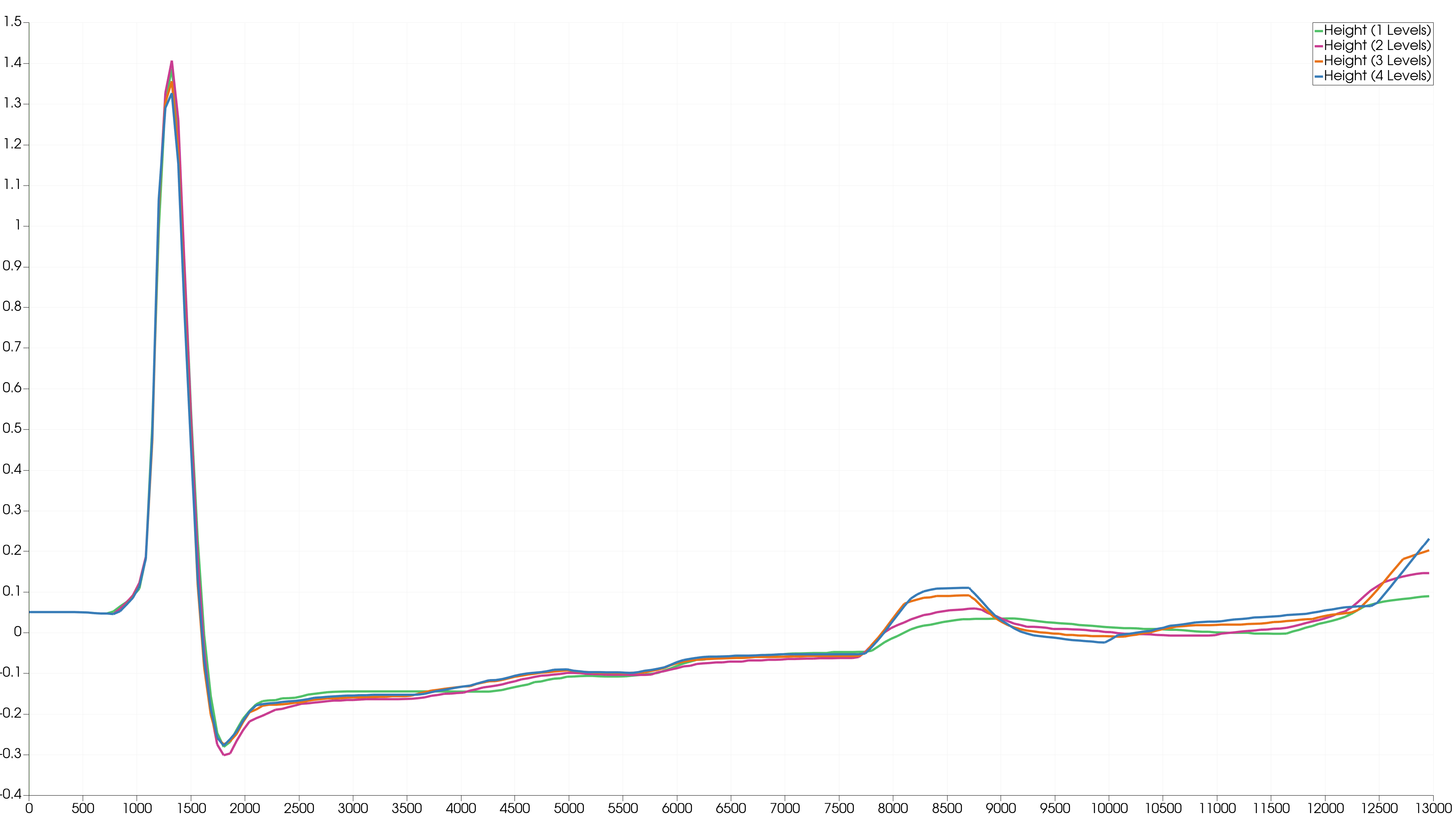
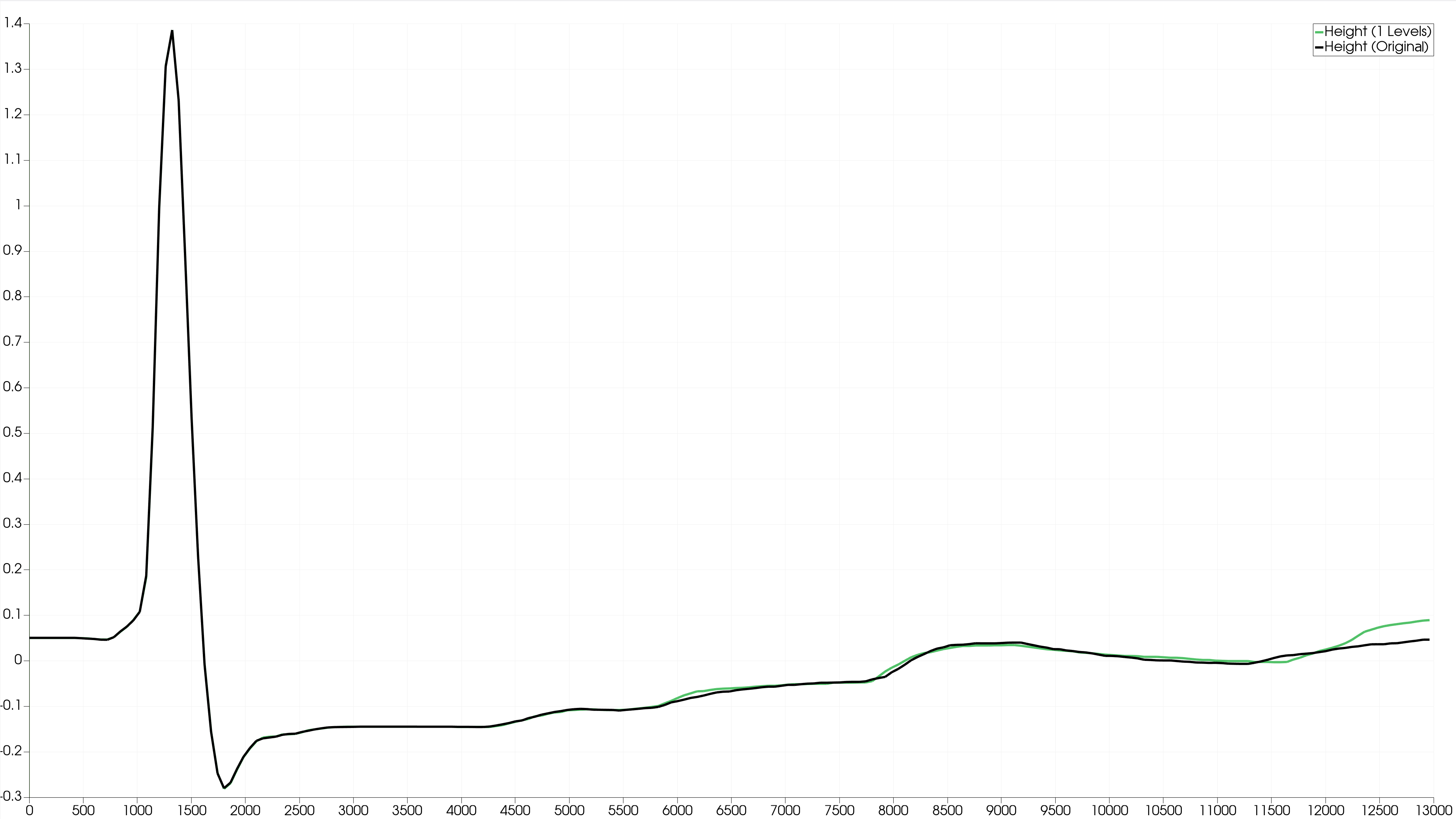
We check the wave height to visually compare the increase in accuracy per level. We plotted the water level of two stations, marked with a cross in the image below.
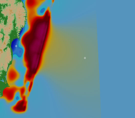
The stations are plotted over time using the output data from the benchmark. Station 1 is the marker close to shore and Station 2 is the marker to the right of the displaced wave.
Station 1
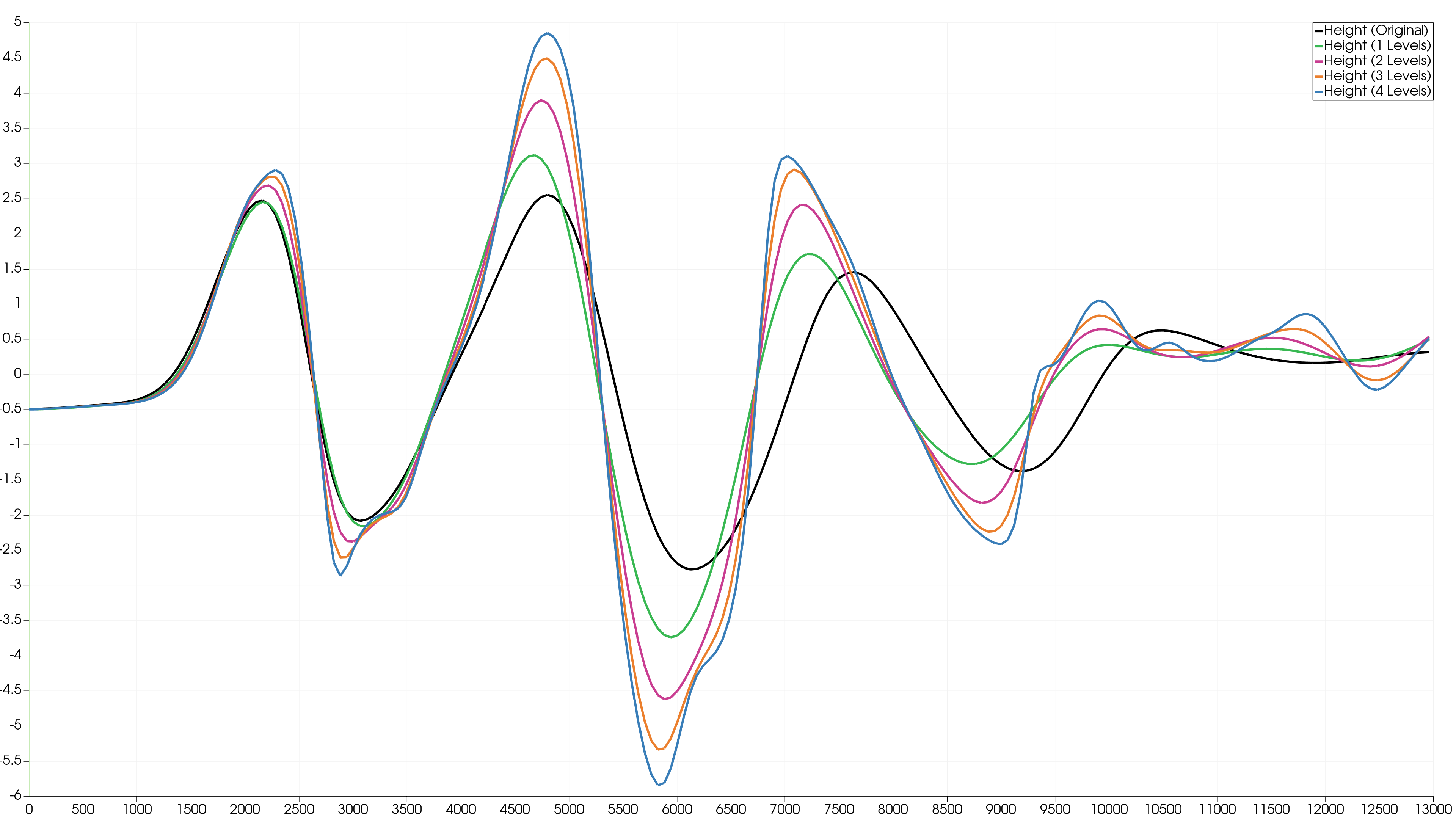
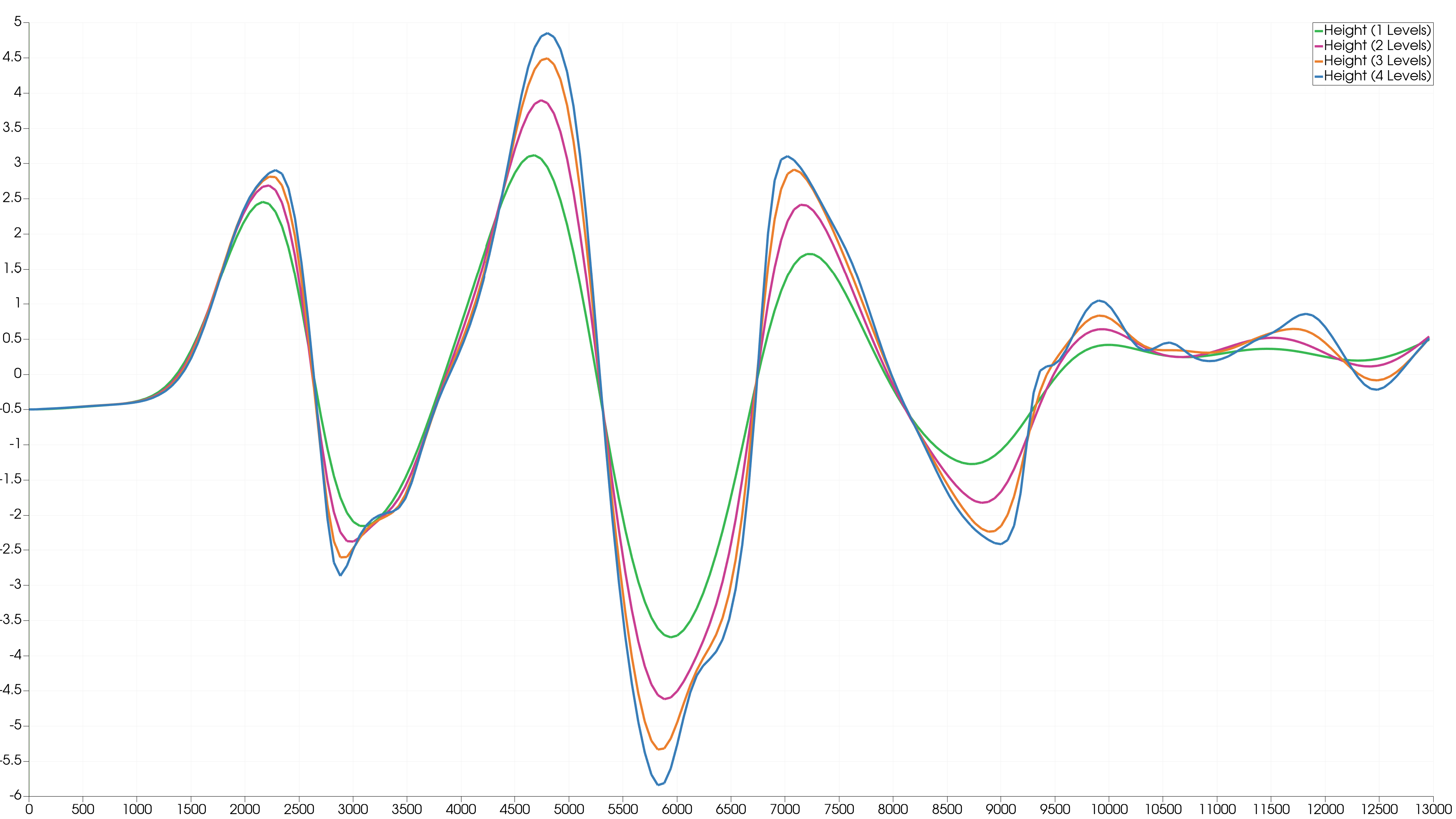
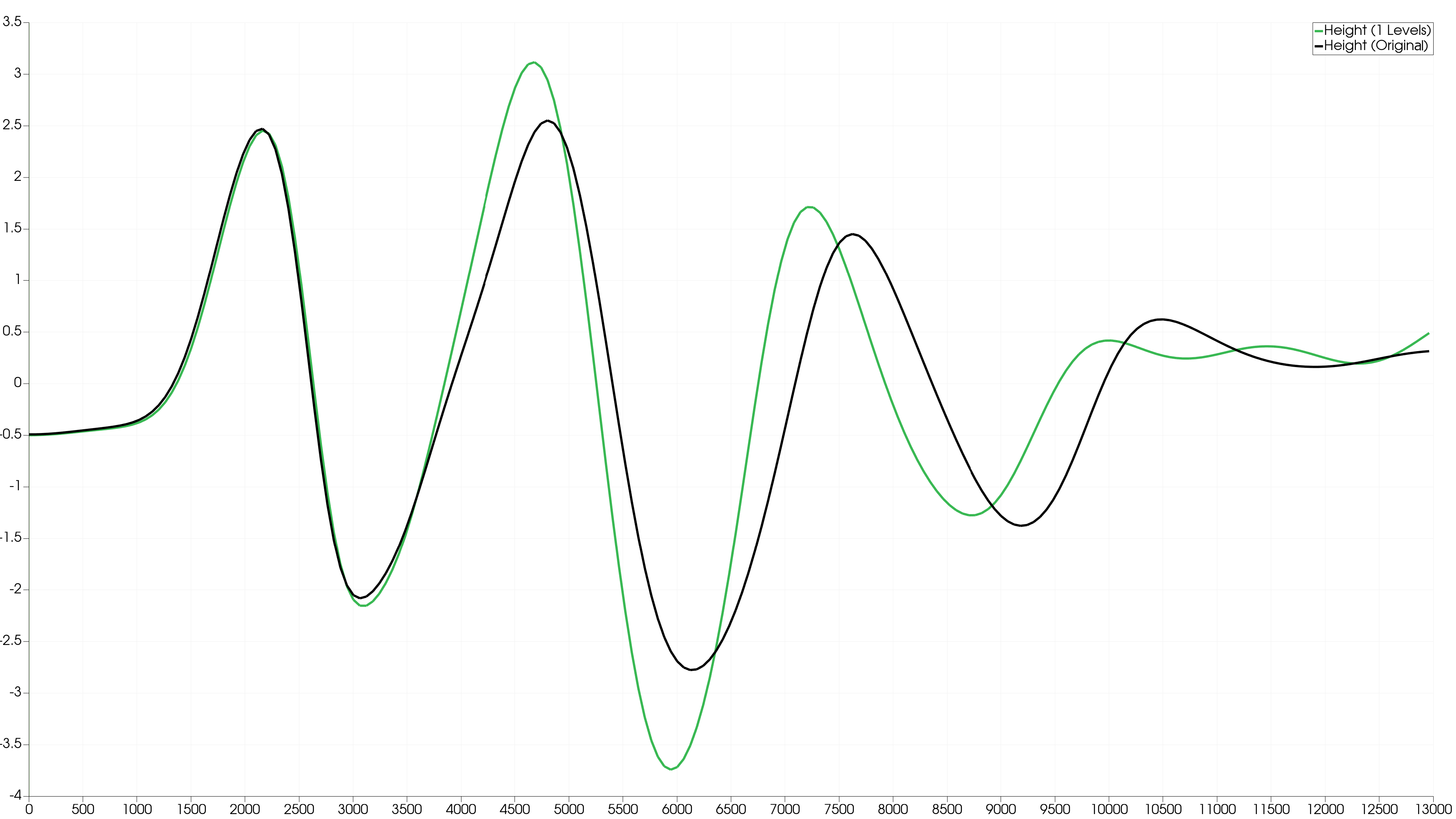
There is a significant difference between the original plot and the AMR Level 1 plot, which are both theoretically identical. This could be due to a shifted initialisation of the bathymetry or simply an interpolation error at the station location by ParaView as our AMR code uses a different format to output the simulation.
We can see a difference in the water level as the number of AMR levels used increases, especially the AMR 4 Levels plot is much more detailed compared to the AMR 1 Level plot. The more levels used, the more irregular the curve becomes. This is because we are in the coastal region, where the water interacts very much, and the simulation can handle rapid changes with more precision.
Station 2
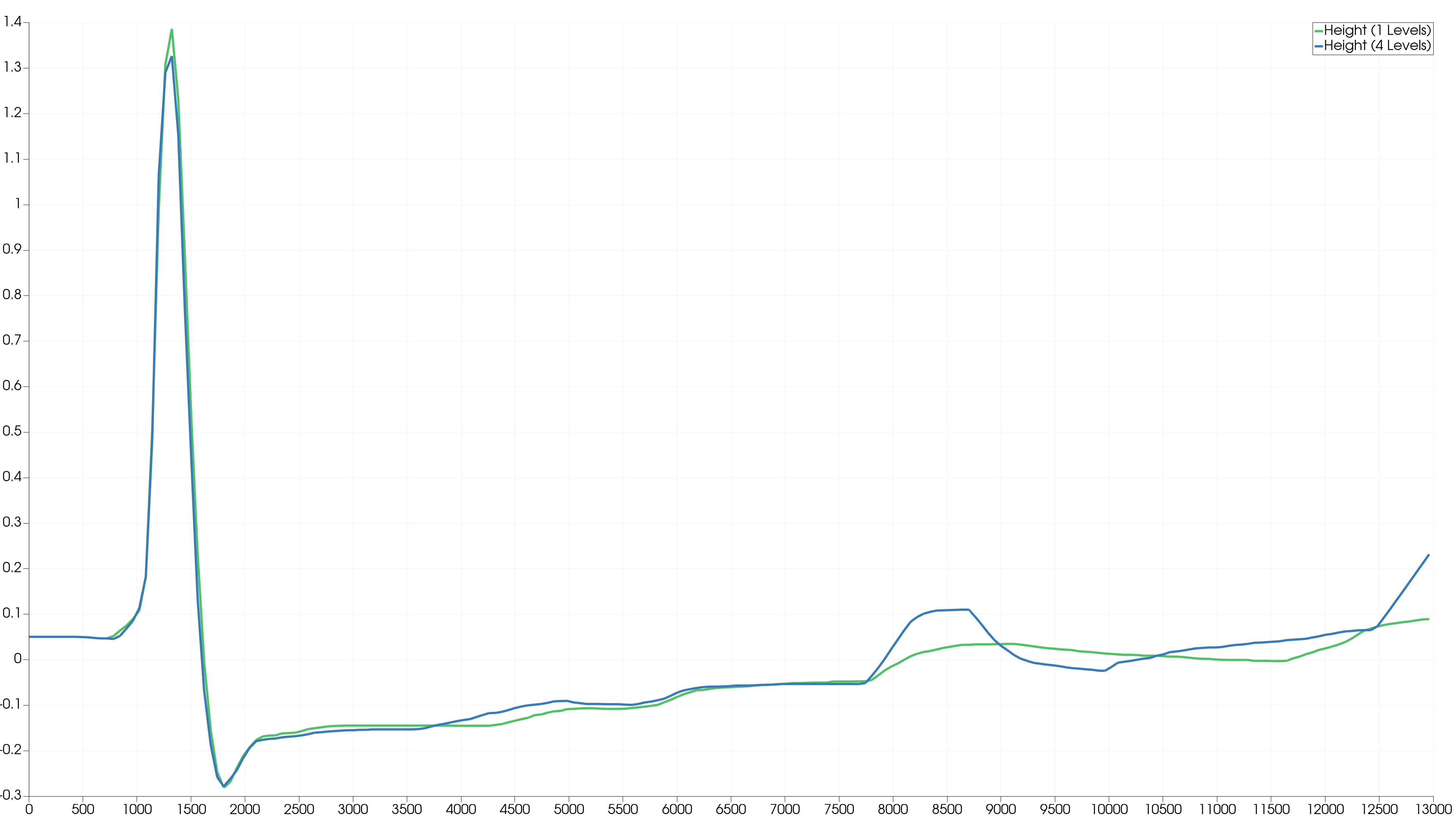
The differences in the seconds stations are not very noticeable. This is because the water is not very hectic and we have a long wave travelling to the right. Only at simulation time 8000 seconds a significant difference can be seen between 1 and 4 Levels. Apparently there is a change at station 2 at this time which could only be taken into account by a high level of refinement.
AMR Tsunami
These videos show the rendered tsunami for different levels of refinement using the output data from the benchmark. Some small difference in wave height can be observed across the videos. The bottom right color legend ranges from -6 to 20 and color the waves. The color legend in the top right corner is a snippet from -1 to 1 of the legend below.
The last video shows the levels of refinement created and merged by AMReX. Here we have used 4 AMR levels.
The criteria yields visually a very good level of refinement near the shore and at the moving waves.
The shore is preferred by the criteria because it has high waves and high velocity due to reflections.
11.6 Building & Running the AMR Project
The requierements and building process are the same as in Building the Project.
Running the Simulation
The executables have been build in to the ../Tsunami-Simulation/build directory with their corresponding name.
E.g. For simulation the executable name would be simulation (or simulation.exe on Windows), etc.
All the executables can be found in ../Tsunami-Simulation/build.
The available executables are simulation, sanitize, test, sanitize_test and test_middle_states.
Note
They are only available when build with their respective --target
E.g. the simulation executable can be run with the following command:
./simulation
Or on Windows with
./simulation.exe
Important
The AMR project uses a settings file inputs.amrex to configure the simulation, which is located in root/resources/inputs.amrex.
Simulation Output
The output of the simulation consists of multiple plot folders.
The files are stored in a separate solutions/ folder, which is located in the working directory of the executable.
Visualization
“There are several visualization tools that can be used for AMReX plotfiles. The standard tool used within the AMReX-community is Amrvis, a package developed and supported by CCSE that is designed specifically for highly efficient visualization of block-structured hierarchical AMR data. Plotfiles can also be viewed using the VisIt, ParaView, and yt packages. Particle data can be viewed using ParaView.”[17]
Here you can find information how to visulaize.
Contribution
All team members contributed equally to the tasks.